I n d i v i d u a l H o u s e h o l d B e h a v i o u r M o d e l l i n g
535
Results and verification
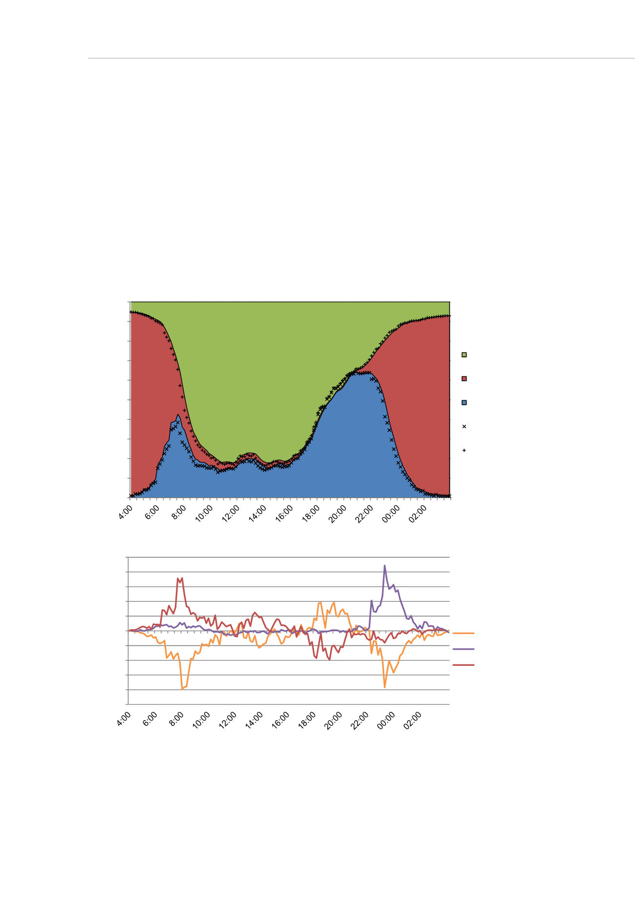
The average output of the occupancy model is shown in
. The area under the
lower curve represents the fraction of people who are present and awake at a certain
time; the area between the lower and the upper curve shows us the fraction of people
who are asleep; the area above the upper curve illustrates the group of people who are
absent. The coloured areas represent the modelled results, whereas the crosses show
the measured data from the TUS data. The deviations between modelled and measured
data are presented in
, where each curve represents an occupancy state. We
can observe that the largest deviations occur when the curves are steep. This is most
likely due to the fact that we took the average over three time steps to calculate the
probability matrices. Between 4 AM and 10 PM the largest deviations occur between
being ‘absent’ or ‘present and awake’. From 10 PM to 4AM the largest differences occur
between ‘present and awake’ and ‘present and asleep’. Overall, there is a close
correspondence between the measured and modelled data.
figure 8: (a) aggregated occupancy profile of a single, full time working person on a weekday after
10000 simulations, (b) absolute deviation between measured and modelled data
0
0.1
0.2
0.3
0.4
0.5
0.6
0.7
0.8
0.9
1
Degree of Occupancy (-)
Time (h)
absent (model)
present and asleep
(model)
present and active
(model)
present and active
(measured)
present and asleep
(measured)
-0.1
-0.08
-0.06
-0.04
-0.02
0
0.02
0.04
0.06
0.08
0.1
Deviation measured-modeled
Time (h)
present and awake
present and asleep
absent


